Linear_model

Build a linear regression model

Steps involved

Understanding the Data
Reading the data in
Data Exploration
Simple Regression Model

import matplotlib.pyplot as plt
import pandas as pd
import pylab as pl
import numpy as np
%matplotlib inline

url="https://s3-api.us-geo.objectstorage.softlayer.net/cf-courses-data/CognitiveClass/ML0101ENv3/labs/FuelConsumptionCo2.csv"
df=pd.read_csv(url)
df.head(5)

	MODELYEAR	MAKE	MODEL	VEHICLECLASS	ENGINESIZE	CYLINDERS	TRANSMISSION	FUELTYPE	FUELCONSUMPTION_CITY	FUELCONSUMPTION_HWY	FUELCONSUMPTION_COMB	FUELCONSUMPTION_COMB_MPG	CO2EMISSIONS
0	2014	ACURA	ILX	COMPACT	2.0	4	AS5	Z	9.9	6.7	8.5	33	196
1	2014	ACURA	ILX	COMPACT	2.4	4	M6	Z	11.2	7.7	9.6	29	221
2	2014	ACURA	ILX HYBRID	COMPACT	1.5	4	AV7	Z	6.0	5.8	5.9	48	136
3	2014	ACURA	MDX 4WD	SUV - SMALL	3.5	6	AS6	Z	12.7	9.1	11.1	25	255
4	2014	ACURA	RDX AWD	SUV - SMALL	3.5	6	AS6	Z	12.1	8.7	10.6	27	244

df.columns

Index(['MODELYEAR', 'MAKE', 'MODEL', 'VEHICLECLASS', 'ENGINESIZE', 'CYLINDERS',
       'TRANSMISSION', 'FUELTYPE', 'FUELCONSUMPTION_CITY',
       'FUELCONSUMPTION_HWY', 'FUELCONSUMPTION_COMB',
       'FUELCONSUMPTION_COMB_MPG', 'CO2EMISSIONS'],
      dtype='object')

df.shape

(1067, 13)

df.info()

<class 'pandas.core.frame.DataFrame'>
RangeIndex: 1067 entries, 0 to 1066
Data columns (total 13 columns):
MODELYEAR                   1067 non-null int64
MAKE                        1067 non-null object
MODEL                       1067 non-null object
VEHICLECLASS                1067 non-null object
ENGINESIZE                  1067 non-null float64
CYLINDERS                   1067 non-null int64
TRANSMISSION                1067 non-null object
FUELTYPE                    1067 non-null object
FUELCONSUMPTION_CITY        1067 non-null float64
FUELCONSUMPTION_HWY         1067 non-null float64
FUELCONSUMPTION_COMB        1067 non-null float64
FUELCONSUMPTION_COMB_MPG    1067 non-null int64
CO2EMISSIONS                1067 non-null int64
dtypes: float64(4), int64(4), object(5)
memory usage: 108.5+ KB

cdf = df[['ENGINESIZE','CYLINDERS','FUELCONSUMPTION_COMB','CO2EMISSIONS']]
cdf.head(9)

	ENGINESIZE	CYLINDERS	FUELCONSUMPTION_COMB	CO2EMISSIONS
0	2.0	4	8.5	196
1	2.4	4	9.6	221
2	1.5	4	5.9	136
3	3.5	6	11.1	255
4	3.5	6	10.6	244
5	3.5	6	10.0	230
6	3.5	6	10.1	232
7	3.7	6	11.1	255
8	3.7	6	11.6	267

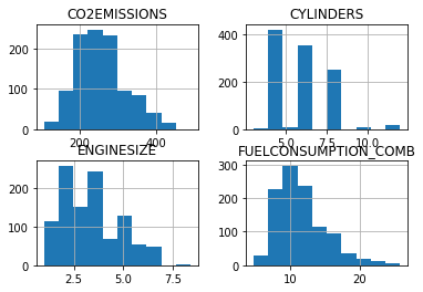
viz = cdf[['CYLINDERS','ENGINESIZE','CO2EMISSIONS','FUELCONSUMPTION_COMB']]
viz.hist()
plt.show()

png

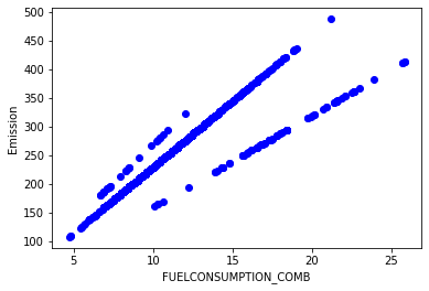
plt.scatter(cdf.FUELCONSUMPTION_COMB, cdf.CO2EMISSIONS,  color='blue')
plt.xlabel("FUELCONSUMPTION_COMB")
plt.ylabel("Emission")
plt.show()

png

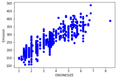
plt.scatter(cdf.ENGINESIZE, cdf.CO2EMISSIONS,  color='blue')
plt.xlabel("ENGINESIZE")
plt.ylabel("Emission")
plt.show()

png

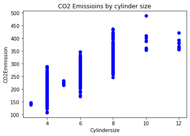
plt.scatter(cdf.CYLINDERS, cdf.CO2EMISSIONS,  color='blue');
plt.xlabel('Cylindersize')
plt.ylabel('CO2Emmission')
plt.title("CO2 Emissioins by cylinder size");
plt.show()

png

#create a random test and train set we will created using numpy arrays
msk = np.random.rand(len(df)) < 0.8
train = cdf[msk]
test = cdf[~msk]

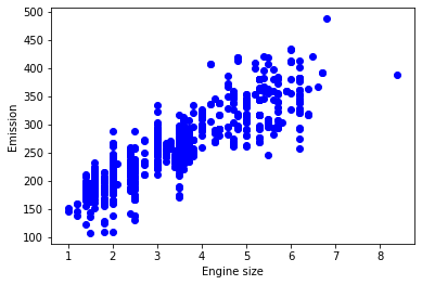
plt.scatter(train.ENGINESIZE, train.CO2EMISSIONS,  color='blue')
plt.xlabel("Engine size")
plt.ylabel("Emission")
plt.show()

png

Modelling

from sklearn import linear_model
regr=linear_model.LinearRegression()
train_x=np.asanyarray(train[['ENGINESIZE']])
train_y=np.asanyarray(train[['CO2EMISSIONS']])
regr.fit(train_x,train_y)
print("coefficents",regr.coef_)
print('intercept',regr.intercept_)

coefficents [[39.11866973]]
intercept [125.8818042]

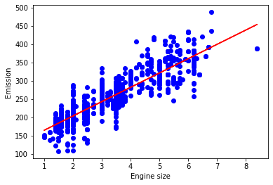
plt.scatter(train.ENGINESIZE, train.CO2EMISSIONS,  color='blue')
plt.plot(train_x,regr.coef_*train_x+regr.intercept_,'-r')

plt.xlabel("Engine size")
plt.ylabel("Emission");
plt.show()

png

Evaluation

we compare the actual values and predicted values to calculate the accuracy of a regression model. Evaluation metrics provide a key role in the development of a model, as it provides insight to areas that require improvement.

There are different model evaluation metrics, lets use MSE here to calculate the accuracy of our model based on the test set:

Mean absolute error: It is the mean of the absolute value of the errors. This is the easiest of the metrics to understand since it’s just average error.
Mean Squared Error (MSE): Mean Squared Error (MSE) is the mean of the squared error. It’s more popular than Mean absolute error because the focus is geared more towards large errors. This is due to the squared term exponentially increasing larger errors in comparison to smaller ones.
Root Mean Squared Error (RMSE): This is the square root of the Mean Square Error.
R-squared is not error, but is a popular metric for accuracy of your model. It represents how close the data are to the fitted regression line. The higher the R-squared, the better the model fits your data. Best possible score is 1.0 and it can be negative (because the model can be arbitrarily worse).

from sklearn.metrics import r2_score

test_x = np.asanyarray(test[['ENGINESIZE']])
test_y = np.asanyarray(test[['CO2EMISSIONS']])
test_y_hat = regr.predict(test_x)
print("Mean absolute error: %.2f" % np.mean(np.absolute(test_y_hat - test_y)))
print("Residual sum of squares (MSE): %.2f" % np.mean((test_y_hat - test_y) ** 2))
print("R2-score: %.2f" % r2_score(test_y_hat , test_y) )

Mean absolute error: 20.54
Residual sum of squares (MSE): 763.95
R2-score: 0.69

Lets check if multinear model will be a better fit

from sklearn.preprocessing import PolynomialFeatures
from sklearn import linear_model

train_x=np.asanyarray(train[['ENGINESIZE']])
train_y=np.asanyarray(train[['CO2EMISSIONS']])

test_x=np.asanyarray(test[['ENGINESIZE']])
test_y=np.asanyarray(test[['CO2EMISSIONS']])

poly= PolynomialFeatures(degree=2)
train_x_poly=poly.fit_transform(train_x)
train_x_poly

array([[ 1.  ,  2.  ,  4.  ],
       [ 1.  ,  2.4 ,  5.76],
       [ 1.  ,  1.5 ,  2.25],
       ...,
       [ 1.  ,  3.2 , 10.24],
       [ 1.  ,  3.  ,  9.  ],
       [ 1.  ,  3.2 , 10.24]])

clf=linear_model.LinearRegression()
train_y_=clf.fit(train_x_poly,train_y)
print("coefficents",regr.coef_)
print('intercept',regr.intercept_)

coefficents [[ 0.         50.205751   -1.46911758]]
intercept [108.27018134]

from sklearn.metrics import r2_score

test_x_poly = poly.fit_transform(test_x)
test_y_ = clf.predict(test_x_poly)

print("Mean absolute error: %.2f" % np.mean(np.absolute(test_y_ - test_y)))
print("Residual sum of squares (MSE): %.2f" % np.mean((test_y_ - test_y) ** 2))
print("R2-score: %.2f" % r2_score(test_y_ , test_y) )

Mean absolute error: 20.58
Residual sum of squares (MSE): 756.06
R2-score: 0.70

shanmukha eeti